Chapter 13 Main effects and interactions
The last few chapters covered the idea of mean group differences, or evaluating whether there is a significant difference between two or more groups. This ability to examine differences between groups is at the foundation of many experiments, with the idea that we can actually see what independent variables may cause changes in dependent variables.
The idea that changes in an independent variable causes a change in a dependent variable is nice, but it’s way too simple for most scientific studies today. There’s a lot of complexity in the world, especially when dealing with people, and that complexity makes things messy.
One example was early research looking at how stress affected performance. The earliest experiment in social psychology (Triplett (1898)) wanted to examine why bicyclers tend to pedal faster when they are in groups rather than being alone. Triplett considered many options in the experiment, including some that we know are true, such as reduced wind resistance, and some that sound quite strange today. One example was “the possibility that the strained attention given to the revolving wheel of the pacing machine in front produces a sort of hypnotism and that the accompanying muscular exaltation is the secret of the endurance.” (Triplett (1898), p. 515).
What Triplett found out was that the stress of having other people working with a person made them work faster. He measured this by having people reel fishing reels and found they reel faster when they were with others. This concept, dubbed social facilitation, is a major theory in social psychology.
However, I’m sure you don’t always think an audience makes you perform better. Many people choke in clutch situations, or freeze when the audience is at their highest.
This kind of pattern happens a lot in behavioral research, where some findings contradict others. It’s a tendency that makes some people want to question science, but for others (like me), it’s part of the beauty of science. Contradictory findings usually indicate that the truth is much more complex than a simple cause and effect.
##Moderators and moderation
To explain findings that seem to be counter-intuititve, we often can consider the idea of a third variable, called a moderator. A moderator is a variable which alters the relatinoship between two other variables. Put another way, an independent variable affects a dependent variable differently, depending on different conditions for the moderator. Moderation is what we call it when a moderator affects a relationship between an independent variable and dependent variable.
Here are some statements that indicate moderation: * Ice cream only increases happiness in summer. Ice cream is the IV, happiness is the DV, and season is the moderator * Listening to m
In other experiments, we may have multiple independent variables, and it’s not clear what is a moderator and what is an independent variable. In these experiments, we might think that both of the variables contribute to the effects in the dependent variable.
For example, we might have the theory that the best way to treat depression is to combine cognitive-behavioral therapy (CBT) and drug therapy. We set up an experiment with four different conditions (no treatment, CBT alone, drug therapy alone, and both CBT and drug therapy). In this case, we have two different independent variables, whether a person receives CBT and whether a person receives drug therapy.
13.1 Factoral design
This kind of logic is also expressed as factoral design, which is the foundation of multivariate ANOVA and is true in many research methods. This is a topic best covered in an research methods textbook, so you should consult one of those if you have more questions. However, I want to give an overview of this, before discussing how this is used in multivariate ANOVA.
A factoral design has two or more variables, which are called factor. Each factor has two or more levels, which are different conditions, within a factor.
A factor is the variable we are interested in examining. For example, one of the factors in the depression treatment experiment mentioned above is CBT treatment. There are two levels in this, yes and no. Did a patient receive CBT or did they not receive CBT? The second factor is drug therapy. Did a patient receive drug therapy or did they not receive drug therapy.
When we discuss factoral designs, we explain them as follows. A 2x2 (say two by two) design has two factors, each with two levels. A 3x5 (say three by five) design has two factors, one factor having 3 levels and one having 5 levels. A 2x2x2 design has three factors, each having two levels. The various combinations of factors are called cells.
13.2 Main effects
The first type of effects we consider in a factoral design are the main effects or differences in the means for the different levels in a single factor, regardless of the other factors.
Let’s take the example above about treating depression. There are two factors, CBT treatment and drug treatment. Each of those factors can have a main effect. The main effect of CBT treatment measures whether there is an any difference between the different conditions of CBT treatment. In this case, there are only two different treatment cases, yes or no. A significant main effect would indicate that the difference between those two means is large enough that it is unlikely it arose by chance alone.
Let’s take the following example table:
| Level of Depression | CBT | No CBT | Mean |
|---|---|---|---|
| Drug | 2 | 4 | 3 |
| No Drug | 4 | 6 | 5 |
| Mean | 3 | 5 | 4 |
In this case, we have to look at each main effect separately. First, we’ll look at the main effect of CBT/No CBT. The mean for the CBT group is 3 and the mean for the No CBT group is 5. Is that a signifcant difference? We would have to do an ANOVA to tell, but we’ll assume that any difference is significant. What this means is that regardless of whether a person received a drug or not, the CBT group is lower than the No CBT group.
The same pattern is true for the Drug/No Drug factor. The mean for Drug is 3 whereas the mean for the No Drug group is 5. Regardless of whether a person received CBT, the Drug group had lower symptom severity than the no drug group.
13.3 Interactions
An interaction is whether the effect of one variable depends on the other variable. There are a lot of possible ways this can happen. I’m going to describe some different examples, and then try to show how it happens in the next section to show how you can visualize interactions.
Example 1: different patterns for different groups. Imagine if you had a study where you looked at how people who were very addicted to caffeine (need 3 cups or more of coffee a day) and how people who never drink caffeine respond to a cognitive test when given caffeine. You might get data like this:
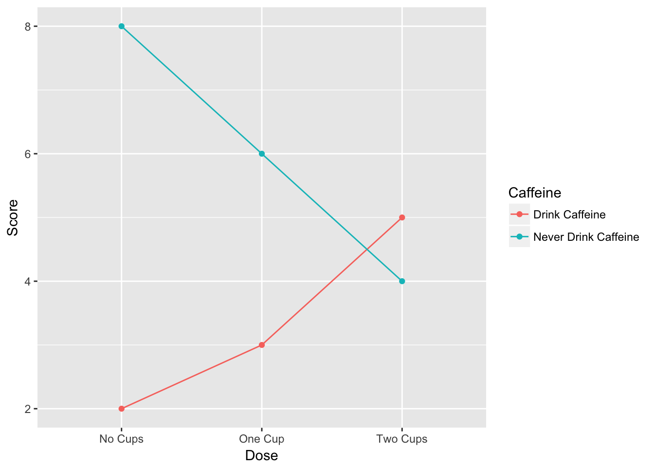
## Using Score as value column: use value.var to override.| Caffeine | No Cups | One Cup | Two Cups |
|---|---|---|---|
| Drink Caffeine | 2 | 3 | 5 |
| Never Drink Caffeine | 8 | 6 | 4 |
There are two different patterns here. For the caffeine group, more caffeine leads to better performance. For the no-caffeine group, more caffeine leads to worse performance.
Since these lines cross in the line graph, you get what is called a crossover interaction, which is powerful evidence for an interaction. Not all interactions are crossover interactions and just because the lines cross, doesn’t mean the interaction is significant. However, this is powerful evidence that an interaction may be apparent.
Example 2: An effect occurs only when two variables are present
In a famous experiment, Schacter and Singer explored how arousal can affect emotions. They tested the theory that a person who is aroused, without knowing why they are aroused, will misattribute that arousal to their circumstances. In an example similar to their study, researchers gave either placebo or adrenaline shots to two groups. One group was told these shots were vitamin shots while the other group were told the shots were adrenaline shots. Then they measured the degree of arousal participants had. The results were similar to this.
e = data.frame(Shot = rep(c("Adrenaline","Placebo"),2),`Participants were told` = c('Vitamin Shot','Vitamin Shot','Adrenaline Shot','Adrenaline Shot') ,`Misattribution of Arousal` = c(7,1,1,1))

ggplot(e, aes(x = Shot, y = Misattribution.of.Arousal, group = Participants.were.told, color = Participants.were.told)) + geom_line(stat = "identity") + geom_point(stat = "identity")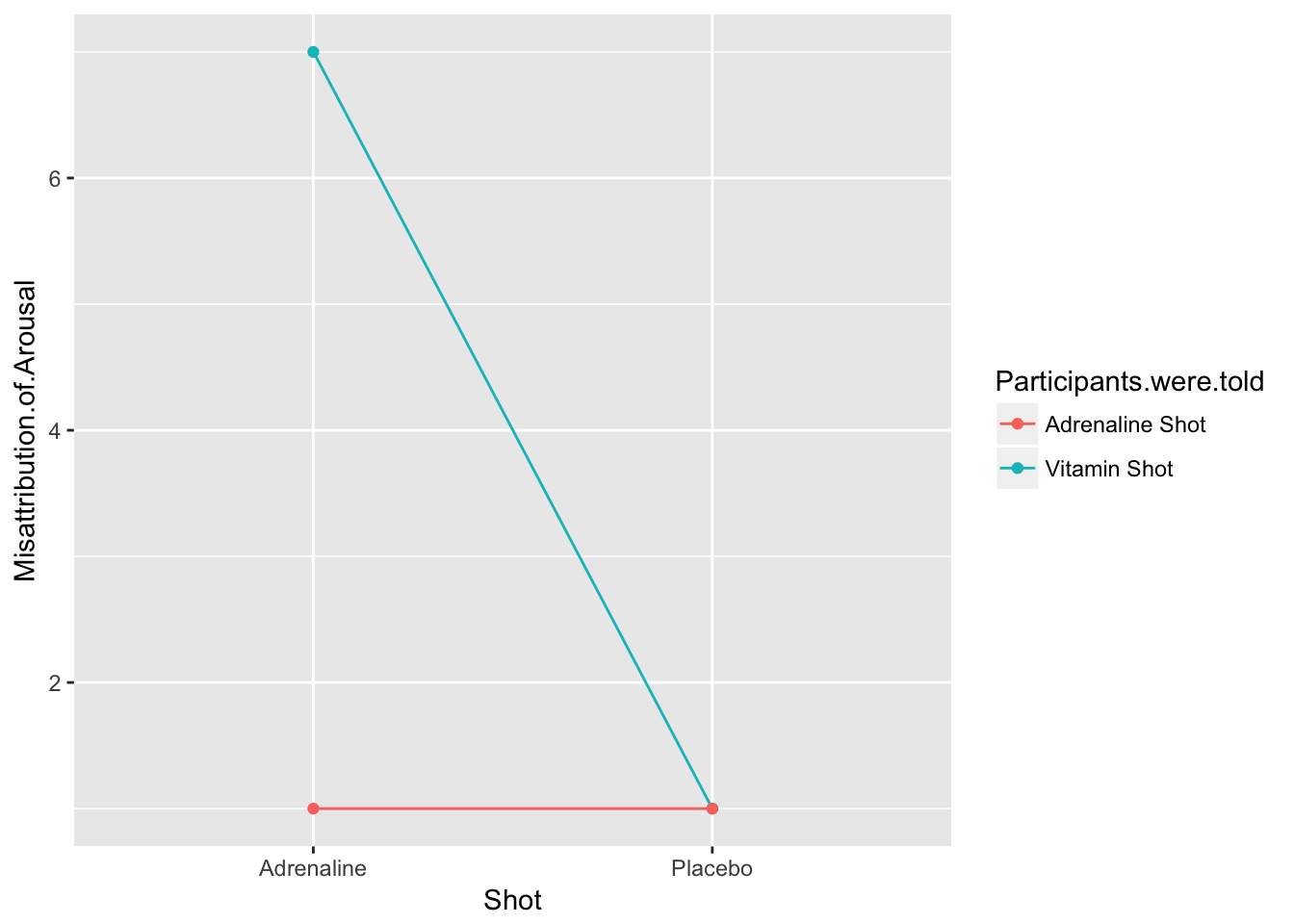
## Using Misattribution.of.Arousal as value column: use value.var to override.| Shot | Adrenaline Shot | Vitamin Shot |
|---|---|---|
| Adrenaline | 1 | 7 |
| Placebo | 1 | 1 |
Notice in this case, there is only major misattribution of arousal when the participants were told the shot was a vitamin shot and it really had adrenaline. This kind of interaction is common when you require two factors to have an effect, and only one factor does not produce an interaction.
Notice in this case, there would also be significant main effects. The mean of the adrenalne group (3.5) is higher than the placebo group (1), regardless of what kind of shot a person received. Likewise, the mean of the group told the shot was a placebo (3.5) was higher than the mean of the group told it was an adrenaline shot.
These main effects are qualified by the interaction. What this means is that they may be significant main effects, but they are caused by the interaction of the two variables, rather than each factor alone.
13.4 Main effects and no interactions
13.5 Interactions qualifying main effects
Whenever there are significant intearctions
Andrade, Jackie. 2010. “What Does Doodling Do?” Applied Cognitive Psychology 24 (1). Wiley Online Library: 100–106.
Bouvard, Véronique, Dana Loomis, Kathryn Z Guyton, Yann Grosse, Fatiha El Ghissassi, Lamia Benbrahim-Tallaa, Neela Guha, Heidi Mattock, and Kurt Straif. 2015. “Carcinogenicity of Consumption of Red and Processed Meat.” The Lancet Oncology 16 (16). Elsevier: 1599–1600. https://doi.org/10.1016/S1470-2045(15)00444-1.
Mangel, Mark, and Francisco J Samaniego. 1984. “Abraham Wald’s Work on Aircraft Survivability.” Journal of the American Statistical Association 79 (386): 259–67. https://doi.org/10.1080/01621459.1984.10478038.
Nigrini, Mark J. 1996. “A Taxpayer Compliance Application of Benford’s Law.” The Journal of the American Taxation Association 18 (1). American Accounting Association: 72.
Triplett, Norman. 1898. “The Dynamogenic Factors in Pacemaking and Competition.” The American Journal of Psychology 9 (4). JSTOR: 507–33.
References
Triplett, Norman. 1898. “The Dynamogenic Factors in Pacemaking and Competition.” The American Journal of Psychology 9 (4). JSTOR: 507–33.